Why you may predict distribution shifts in generalization, and how

14 minute read

Distribution shift is a key issue in generalizing statistical inference from one population to another, an important task in many fields. This post discusses recent progress in understanding, modeling, and addressing real distribution shifts supported by both empirical evidence and theoretical modeling. The discussion is based on two papers:

J., Guo and Rothenhäusler (2023). Diagnosing the role of observable distribution shift in scientific replications. [Arxiv] [Dataset] [R package]
J., Egami, and Rothenhäusler (2024). Beyond reweighting: On the predictive role of covariate shift in effect generalization. [Arxiv] [Reproduction code]

We will see how unknown components in real distribution shifts can be predicted, why this could make sense, and how it would be useful in the future.

Distribution shifts in generalization

Generalization tasks often rely on data from a source population to make inferences about a target population with only partial information.

As a running example, consider an educational intervention tested in a California high school (source population), where both student characteristics (e.g., age, income, grades) and outcomes are observed. Researchers may then seek to predict how the intervention would perform in a New York high school (target population), where only student characteristics are available. Since we haven’t yet collected the target outcomes, we have no idea how students in New York may differ from students in California. How to address such differences? How far can the effect generalize? These are fundamental questions researchers ask when considering such tasks in many domains.

To formalize, we observe \((X,Y)\) from the source population \(P\), and only the covariates \(X\) from the target population \(Q\). By checking the covariates, we can assess how the NY and CA students differ in ages, family income, and parent education. This is called covariate shift between \(P_X\) and \(Q_X\) (blue part in the figure below). In addition, the distribution of the outcomes \(Y\) given covariates may also differ, which is the conditional shift (red part in the figure below). Since \(P = P_X\otimes P_{Y\mid X}\) and \(Q = Q_X \otimes Q_{Y\mid X}\), the two shifts compose the entire distribution shift.

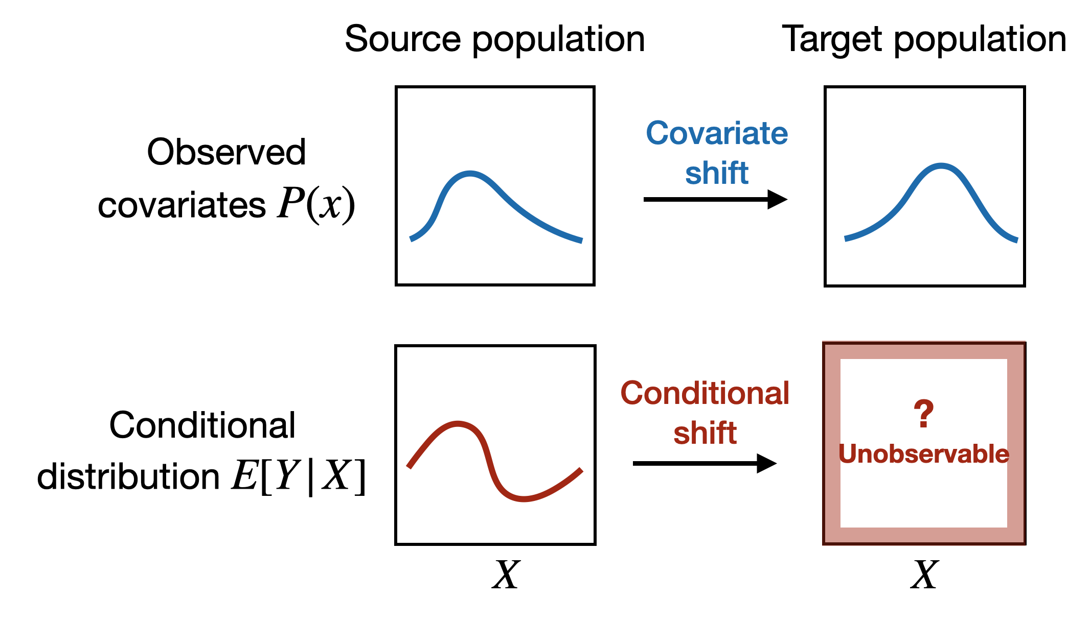
predictive role. — *Distribution shift from source to target populations consists of covariate shift and conditional shift.*

The nature of the two shifts is very different. The covariate shift is estimable since we have data from both places. However, we have no idea how the conditional shift is like. Two students from CA and NY with exactly the same covariate profile may still differ a lot in their behavior due to unmeasured factors. But we never know.

Narrowing the scope

Various distribution shifts occur in many fields. In this post, we restrict the scope to settings where the distribution changes within the support of the source distribution, avoiding scenarios that require extrapolation. Technically, this just means that the density ratio (or Radon-Nikodym derivative) between \(Q\) and \(P\) exists.

Another implicit restriction is that we focus on a kind of natural distribution shifts that are not due to adversarial manipulations. This describes a broad range of settings in generalizing statistical inference in social and biomedical sciences, where the samples are, e.g., human beings, that will not be deliberately altered yet still inevitably differ, and the data collection process is prone to unexpected but non-adversarial changes.

Replication datasets offer a valuable lens to study these shifts (now abundantly available thanks to efforts from the replicability community). Such datasets can be paired studies where a replication study is conducted after the original one [1]. In paper [2], we use two famous large-scale multi-site replication studies, the Many Labs 1 project [3] and the Pipeline project [4], where more than ten research groups across the world independently conduct the same experiments to examine the same set of scientific hypotheses. Such a data collection process removes concerns about publication bias and ensure consistency to the largest extent possible, while providing rich information with multiple sites and hypotheses. While researchers try to ensure consistency, unexpected factors may still lead to subtle differences, making them suitable to examine the realistic shifts we are interested in.

Conditional shift is nontrivial…

To formalize the discussion, we are interested in parameters as function of the underlying distribution, \(\theta(P)\) and \(\theta(Q)\), which are expectations of a test function, i.e., \(\theta(P) = \mathbb{E}_P[\phi(X,Y,T)]\) for some known function \(\phi\), and \(T\in \{0,1\}\) is the treatment indicator. It can be the difference-in-mean for randomized experiments or a paired difference for paired \(t\)-test. With full observations, we can compute estimators \(\hat{\theta}(P)\) and \(\hat{\theta}(Q)\) as sample mean of the test function. To infer \(\theta(Q)\) with only covariates from \(Q_X\), we need assumptions on the unknown \(Q_{Y\mid X}\).

A leading paradigm in the literature is to assume that \(Q_{Y\mid X} = P_{Y\mid X}\), that is, the conditional shift doesn’t exist. This is often called the covariate shift assumption (CSA for short), as it posits that the covariate shift explains away all differences. This is widely employed not only in the generalizability literature but also machine learning areas.

💡 The first question we address is: Is covariate shift assumption real?

To do so, we take all pairs of sites in project, use one as source and one as target, employ existing approaches justified under the CSA to construct prediction intervals (PIs) for \(\hat\theta(Q)\), the target estimate, and then examine the empirical coverage of these PIs. Since these PIs will achieve valid coverage under the CSA, their actual coverage examines the plausibility of the assumption.

Somewhat surprisingly, the distribution shift is real, but the CSA is not. In the figure below, the grey bars in (a) are the empirical coverage of PIs based on the i.i.d. assumption that \(P=Q\). The under-coverage shows the impact of distribution shifts. However, adjusting covariate shifts is also not enough: the green and purple bars are the coverage of those CSA-based PIs, which also under-cover. Panels (b) show estimates for different source studies for a single target study: reweighting to adjust for covariate shift doesn’t necessarily bring the estimates closer to the target.

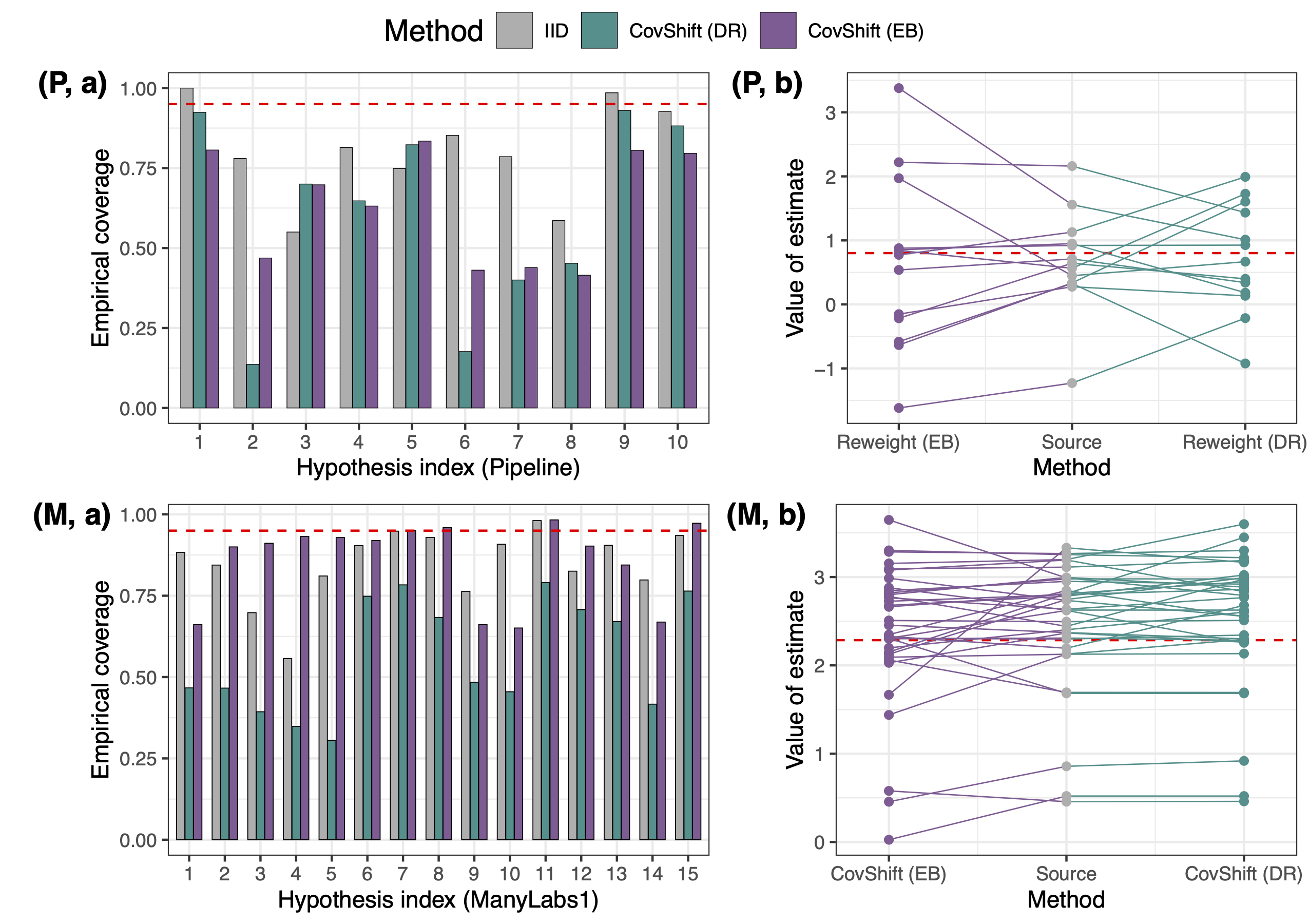
While this finding challenges the sufficiency of CSA, it is actually coherent with some recent empirical investigations on real distribution shifts, in that covariate shift only explains a small proportion of the observed discrepancy. This seems quite pessimistic: the conditional shift is nontrivial, and seems to be “larger” than the covariate shift. How can we address the conditional shift in a real generalization task?

… but it can be bounded!

Fortunately, we have some good news.

💡 Our second finding is: Conditional shift can be bounded, but only with a carefully designed measure.

Let’s first formalize how the two shifts impact the parameter. Note the decomposition

\[\theta(Q)-\theta(P)= \mathbb{E}_Q[\phi] - \mathbb{E}_{P}[\phi] = \underbrace{\big\{ \mathbb{E}_Q[\phi_P(X)] - \mathbb{E}_P[\phi_P(X)]\big\}}_{=:\text{ Covariate shift}} \ + \ \underbrace{\big\{ \mathbb{E}_Q[\phi - \phi_P(X)] \big\}}_{=:\text{ Conditional shift}},\]

where \(\theta_P(x):=\mathbb{E}_P[\phi\mid X]\) is the conditional expectation. The first term is the contribution of covariate shift (which is zero if \(P_X=Q_X\)), and the second term is the contribution of conditional shift (which is zero if \(P_{Y\mid X}=Q_{Y\mid X}\)). The intermediate quantity \(\mathbb{E}_Q[\phi_P(X)]\) is often estimated by reweighting to adjust for covariate shift. In [1], we used this decomposition to diagnose how much of a discrepancy between two studies can be attributed to the two shifts.

However, the above two terms we use in [1] are not good measures of strength of distribution shift, because they are scale-dependent: even with the same strength of perturbation to the probability space, linearly scaling \(\phi\) will lead to different results. So we replace them by standardized measures. For conditional shift, we use

\[\text{Relative conditional shift} = \frac{\mathbb{E}_Q[\phi - \phi_P(X)]}{\text{sd}_P(\phi - \phi_P(X))}.\]

For covariate shift, instead of a similar quantity \(\frac{\mathbb{E}_Q[\phi_P(X)] - \mathbb{E}_P[\phi_P(X)]}{\text{sd}_P(\phi_P(X))}\), we use a stabilized version:

\[\text{Stabilized covariate shift measure} = \sqrt{\frac{1}{L} \sum_{\ell=1}^L \frac{(\mathbb{E}_Q[X_\ell] - \mathbb{E}_P[X_\ell])^2}{\text{Var}_P(X_\ell)}}\]

which permits stable estimation for practical use in generalization.

Next, we take data from all pairs of sites in the replication projects that examine the same hypothesis, and compute the above two measures. We then plot the distribution and pairwise relationships of these measures for various site pairs. The pairwise relation is surprisingly clean: the covariate shift measure upper bounds the conditional shift most of the time across different scenarios. When the conditional shift is larger, the covariate shift also tends to be larger, showing a predictive role. This pattern emerges only after we use the standardized, stabilitized mesures, and you can find explorations of other measures (ignoring either scale invariance or numerical stability) in [2].

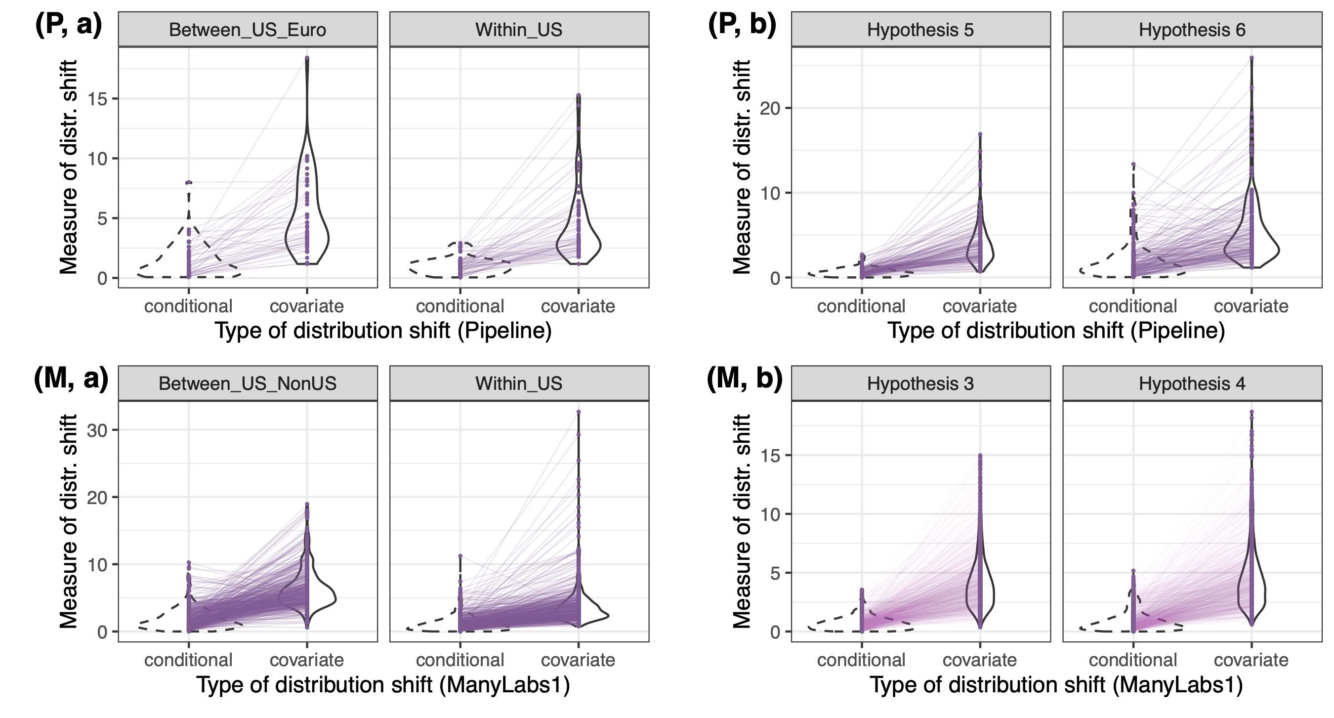
The practical implication of this finding is that, in a real generalization task, you can compute the covariate shift measure, and it’s safe to believe that the unknown conditional shift measure is no greater than it. By definition, this should give you a range of \(\theta(Q)- \mathbb{E}_Q[ \phi_P(X)]\), the remaining discrepancy after you adjust for the covariate shift.

Why this makes sense? Some modeling

So far, the discussion is purely empirical: we just looked at the data, computed some quantities, and found a pattern. Why would this pattern make sense? In what settings the conditional shift might be smaller than the covariate shift? We now provide some theoretical modeling to justify and further understand it.

We model the data collection procedure as a two-stage process. In the first stage, the distribution \(Q\) is created by the nature randomly ``perturbing’’ \(P\). In the second stage, data is drawn i.i.d. from the perturbed distribution \(Q\).

How the distribution is perturbed is key to our results. We will not go into technical details, but roughly speaking, there are forces that randomly bring the probability of tiny pieces of the probability space up and down. Like in the figure below, the probability space of both the covariates and unmeasured factors (impacting the unknown outcomes) is cut into small pieces with equal probability, each of which is perturbed by independent and identically distributed randomness. Taking the grid finer and finer gives our final perturbation model.

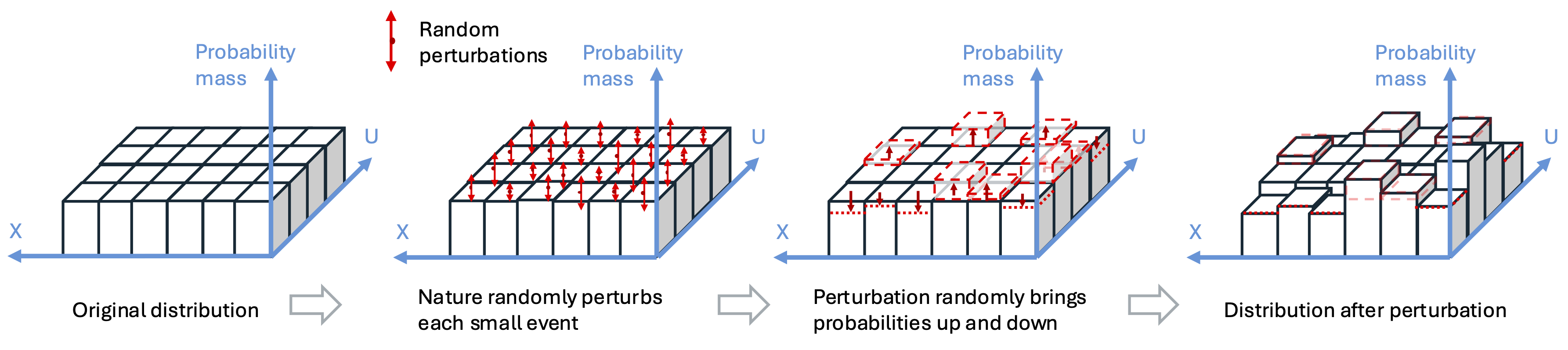
Numerous small pieces of perturbations lead to behavior like central limit theorem in the distribution. We have a distributional CLT which states that the sample mean of any test function \(\psi(\cdot)\) under \(Q\) follows a normal distribution with a distinct asymptotoc variance than \(\text{Var}(\psi(X,Y,T))\).

[Distributional CLT] Under the above distribution shift model, suppose \(Y=g(X,T,U)\) for some unknown \(g(\cdot)\), and \(U\) is unmeasured features. Then, as sample size and the number of grids go to infinity, we have \(s_n^{-1} \left( \hat{\mathbb{E}}_Q[\psi] -\hat{\mathbb{E}}_P[\psi] \right) \stackrel{d}{\rightarrow} \mathcal{N}(0,1)\), where \(\delta_\text{M}^2\) is a constant that measures the strength of perturbation, and \(s_n^2 = \left( \frac{1}{n_P} + \frac{1}{n_Q} \right) \text{Var}_{P}(\psi) + \delta_\text{M}^2 \text{Var}_{P}(\mathbb{E}_P[\psi \mid X,U])\).

Applying the above distributional CLT to the conditional and covariate shift measures, we will have

\[\frac{(\hat{\mathbb{E}}_Q[\psi] - \hat{\mathbb{E}}_P[\psi])^2}{\hat{\text{Var}}_P(\psi)} \stackrel{d}{=} \left(\frac{1}{n_P} + \frac{1}{n_Q} + \delta_M^2 \frac{\text{Var}_{P}(\mathbb{E}_P[\psi \mid X,U])}{\text{Var}_{P}(\psi)} \right) Z_1 + o_P(\delta_M),\]

where \(Z_1\sim \chi^2(1)\), and on the other hand,

\[\frac{(\hat{\mathbb{E}}_Q[X_\ell] -\hat{\mathbb{E}}_P[X_\ell])^2}{\hat{\text{Var}}_{P}(X_\ell)} \stackrel{d}{=} \left(\frac{1}{n_P} + \frac{1}{n_Q} + \delta_M^2 \right) Z_1 + o_P(\delta_M).\]

Since the variance of conditional expectation is smaller than the marginal variance, the first quantity (conditional shift measure) is generally smaller than the second (covariate shift measure), which is what we observe in the datasets.

Let us now discuss some intuitions. Since small pieces are perturbed in an i.i.d. fashion, the perturbation doesn’t favor any direction, creating homogeneous distributional changes across the space. Thus, the distribution of any test function \(g(X,U)\) is perturbed with the same strength. However, since \(Y\) is a function of \((X,U)\) and the treatment indicator \(T\) whose distribution is invariant due to experimentation, it is “downstream” in the data generating process, and its perturbation is weaker than the original perturbations to \((X,U)\).

Empirical validation is often limited (e.g., inference for parameters can never be evaluated in real data), and this is why a good model is important — it allows us to build new methods without empirical validation all the time. A good model should describe the type of shift that indeed happens. Our model is nice because it generates similar patterns that actually occur in the data. Intuitively, it describes scenarios in replication studies or more broadly generalization efforts, where researchers try to keep things consistent but numerous small perturbations still randomly occur, such as subtle changes to the implementation of treatments, small errors in measuring the variables, so on and so forth.

How could this help? Generalization with calibration

We have now demonstrated a predictive role of covariate shift: it can bound and predict the strength of unknown conditional shift. This is justified by both empirical evidence and theoretical modeling. The random distribution shift model seems a good one for describing small, unexpected changes that would happen in generalization tasks.

💡 The final question we address is: How is the predictive role useful, besides scientific understanding?

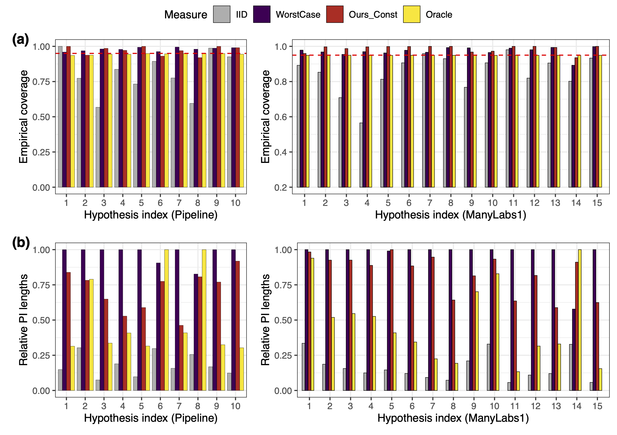
An immediate use is that we can build PIs for the target estimator without any other information. Consider a real generalization task with full data from \(P\) and covariates from \(Q\). We can then compute \(\hat{t}_X\), an estimate of the covariate shift measure, \(\hat{s}_{Y\mid X}\), an estimate of \(\text{sd}_P(\phi - \phi_P(X))\), and \(\hat\theta_w\), an estimate of \(\mathbb{E}_Q[\phi_P(X)]\). The bounding role simply means \(\frac{\| \hat\theta_Q - \hat\theta_w \|}{\hat{s}_{Y\mid X}} \leq \hat{t}_X\) most of the time. Inverting this relation gives a prediction interval

\[[ \hat\theta_w - \hat{t}_X \cdot \hat{s}_{Y\mid X} , ~ \hat\theta_w + \hat{t}_X \cdot \hat{s}_{Y\mid X}]\]

for \(\hat{\theta}(Q)\). The figure below shows the performance of such PIs (red) across all site pairs for each scientific hypothesis. They achieve high coverage with shorter lengths than worst-case bounds that assume adversarial perturbations. (The worst-case bounds assume the KL-divergence between \(Q_X\otimes P_{Y\mid X}\) and \(Q\) is bounded by some \(\eta\); we (unrealistically) calibrate the value of \(\eta\) with all data, and then search for the lower and upper bound of \(\theta(Q)\) under this KL-divergence bound.)

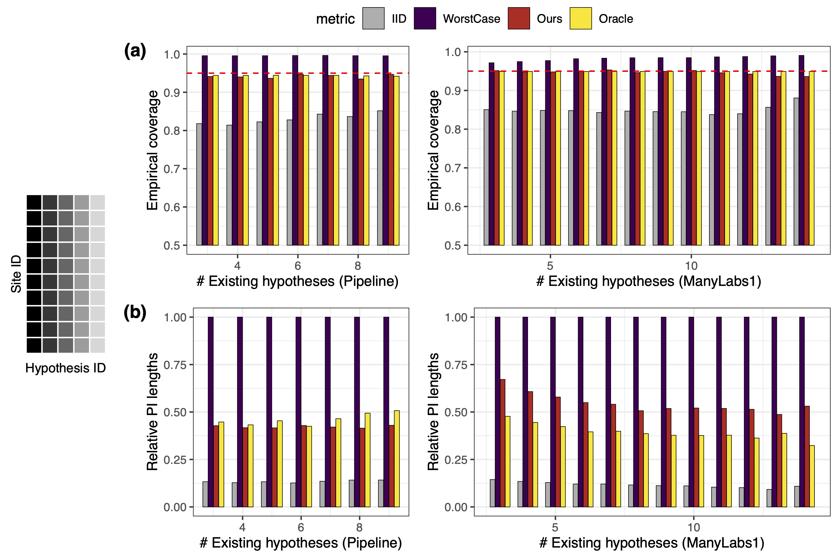
More generally, if external information is available, we may calibrate a high-probability range \([L,U]\) of the distribution shift ratio. Then a prediction interval for \(\hat{\theta}_Q\) would be

\[[ \hat\theta_w + L\cdot \hat{t}_X \cdot \hat{s}_{Y\mid X} , ~ \hat\theta_w + U\cdot \hat{t}_X \cdot \hat{s}_{Y\mid X}].\]

The figure below shows the coverage and length of PIs when \((L,U)\) are calibrated as quantiles of the ratio between the two distribution shift measures for testing other hypotheses in the same sites. We achieve near-exact coverage with drastically shorter PIs. This shows the distribution shift ratio is stable across different contexts, so other datasets are informative of a new generalization task.

Closing remarks

I am really excited about the positive messages on how we may predict the unknown supported by our empirical and theoretical analyses. But I have to be very cautious about the scope these messages apply to: it describes scenarios with no manipulations, so that the probability space is perturbed without favoring any direction.

This restriction motivates future avenues to pursue. For example, when the researcher can emulate the study population, the covariate distribution may be subject to stronger changes yet the conditional distribution is randomly perturbed. Real distribution shifts may be a mixture of controlled and unintended random shifts. A natural question is how to devise estimators and inference procedures in these scenarios.

The idea that unknown shifts can be informed by differences in covariates has promise for wider use. We may use observed covariates to judge the usefulness of different datasets for a specific generalization task. Using multiple datasets could be critical for removing the distributional uncertainty resulted from the random shifts.

Empirically, besides pairwise investigations of generalization performance, is it possible to build a more “global” map for generalizability? With the abundance of multi-site, multi-hypotheses datasets, can we merge different studies to investigate how different sites relate to each other? Is there a “GWAS”-like map [5] for generalizability?

References

[1] J., Guo and Rothenhäusler (2023). Diagnosing the role of observable distribution shift in scientific replications. [2] J., Egami, and Rothenhäusler (2024). Beyond reweighting: On the predictive role of covariate shift in effect generalization.
[3] Klein, Richard A., et al. Investigating variation in replicability. Social psychology (2014).
[4] Schweinsberg, Martin, et al. The pipeline project: Pre-publication independent replications of a single laboratory’s research pipeline. Journal of Experimental Social Psychology 66 (2016): 55-67.
[5] Novembre, John, et al. Genes mirror geography within Europe. Nature 456.7218 (2008): 98-101.